Altair Flux 2019 Release Notes
Essential Information
| Essential information about Flux 2019 |
|---|
|
For Flux 2019 the user has the possibility to be protected by "HWU" protection (Windows and Linux) exclusively. The Legacy protection has been removed. |
In order to use the version HWU, you need:
|
Flux 2019 is available for Windows and Linux OS:
|
| Flux 2019 takes into account several user feedbacks, and 21 issues have been solved in this version. |
| Distributed computing with MPI is available in Flux for Windows and Linux and can be used with PBS. However, qualification on Windows cluster connected with InfiniBand has not been done and Linux clusters is highly recommended for parallel computing. |
| The new feature “Flux starting guide” is only available in Windows (not in Linux). |
| It is now possible to install Flux on Windows or Linux without administrator rights with limited functionalities. |
Minimum memory required:
|
| SPEED import is not available since Flux 2018 version. Please use a previous Flux version to import your SPEED file. |
| The Student Edition of Flux 2019 will be available few weeks after the release of the professional edition. |
New Features
New features dealing with Environment
| New features | Description | |||||||||
|---|---|---|---|---|---|---|---|---|---|---|
| Branding | FluxTM become Altair FluxTM. | |||||||||
| User Mode | A user mode has been implemented. Thus
the user has the choice between 3 modes:
|
|||||||||
| Renaming of the command "Run a python file" | Labels and python command have been changed for
running a python file:
Note: The "legacy" python commands are always compatible
with Flux 2019 and future version.
|
New features dealing with Meshing
| New features | Description |
|---|---|
| Visualize volume elements internal to solids by a cut plane |
Possibility to visualize volume mesh element according to a plan defined by 3 points. 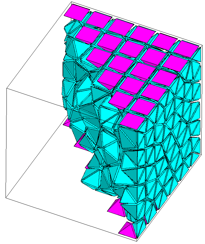 |
| New mesh generator by "Layers" |
This mesh generator, based on the MeshGems-Hybrid module of Distene, is a mixed mesh elements generator in Flux (it creates hexahedra, prisms, pyramids, or tetrahedra). It allows to mesh the skin depth with extruded elements (prisms, hexahedra) and relax the mesh in the remaining volume. It is based on the initial surface mesh of the volume without modifying it. 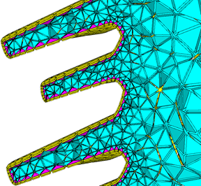 |
| Mesh Import - wire body |
Now, when importing mesh, wire body are also imported into Flux, to allow using line region later. |
| Improvement of shell elements generation with mesh import | The orientation of the current density on the shell bodies in areas was wrong where the surface elements had been merged during the mesh import. The improvement implemented has been to take into account the correct normal vector on these faces (merged surface elements) in the different Flux algorithms. |
New features dealing with Physics
| New features | Description | |||||||||||
|---|---|---|---|---|---|---|---|---|---|---|---|---|
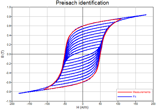
| Preisach Model (Hysteresis) in Beta mode |
A new static vectorial hysteretical model has been developped in
Flux in Beta mode (Supervisor option). This model is
easier to use than the Jiles-Atherton model. The Preisach model
is more powerfull to generate minor loops. This model comes in
two materials.
Note: If you want test and use the fitting tool with the new
hysterical material, please contact the Support.
|
|||||||||||
| Speed up of iron losses computation in post processing |
Some improvements have been done with the new iron losses model, especially for the computation time in postprocessing. |
New features dealing with Solving
| New features | Description |
|---|---|
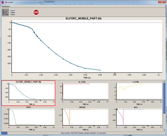
| Result Preview | During the solving, a set of curves are
automatically displayed and give the evolution of the main
quantities in runtime. If the evolution is wrong, the user can stop directly the solving and adjust his model.
|
| Add a Newton-Raphson to fixed point switch for the maximal factor method | For non-linear solving using this relaxation method is now more robust and can improve convergence |
| Simplification of GUI for solving process options |
With Flux 2019, the Linear system solver
options tab has been simplified. In
Standard mode, the user has only to
choose between 2 types of solver before solving:
By doing this, the options have been standardized. The older solvers used in the previous version of Flux stay available through the Advanced mode. This mode can be set using the supervisor. The filtered options are set to a default value. Solving process options are applicable for all physical applications of Flux 2D, 3D and Skew. |
| New initialization method by prediction |
With Flux 2019, a new initialization method of the state variables at the beginning of each time step is proposed to the user. This method consists in computing a predicted solution of the current time step using previous ones to converge faster. |
| Matrix size estimator improvement | The estimation of the matrix size could be excessively overestimated, causing a memory-based error message whereas the solving would have been possible. A fix has been done to reduce the cases of excessive overestimation. |
| Automatic local/distributed solver strategy | An automatic selection between MUMPS local and distributed is done based on the dimension of the problem and the correctness of the user configuration. User can still use manual selection by using « advanced mode ». |
| Ensure compatibility with other batch schedulers (parallel computing) | Commands used for parametric distribution through PBS are now accessible and can be modified, making all Altair Flux/PBS features can now be used with other batch schedulers. |
New features dealing with Post-processing
| New features | Description |
|---|---|
| 3D curve dedicated to rotating machine |
The 3D curve dedicated to rotating machine allows computing a formula values along a computing circle positioned around a rotating machine rotation axis. Those values are collected for a set of time steps (feature available only in Transient Magnetic application). Once collected, the values are represented in a 3D curve having in abscises the time and the angular position along the computing circle. A specific option allows eventually to compute those values in 2D Fourier domain depending on the motor-harmonic and the spatial order. |
New features about dedicated contexts
| New features | Description |
|---|---|
| Context of Data Import/Export |
The data import/export context is a Flux environment dedicated to exchanges between Flux and a third party software. It allows making a weak coupling with another application software:
This context is implemented in Flux since the 2018 version. It is enriched and more robust at each version. In this 2019 version, a thermal export to OptiStruct has been added. |
New features about some added commands
| New features | Description |
|---|---|
| Active scenario |
A new command getActiveScenario() has been implemented to have the possibility to know which solving scenario is ON when opening Flux with PyFlux. For example, the calling of Flux from SimLab is simplified with this new python command. When opening a solved project that has several scenarios, the post-processing operations point to a given step of a scenario. This new getActiveScenario() command allows knowing which one. In a scrip, you have acces to the following command: result = getActiveScenario() print result.name The instance of the active scenario is returned by the command. Reminder: there is a family of commands to control the post-processing in python (see the document How to get the steps of a scenario available from Flux Supervisor) |
| new APIs about user I/O parameters (Groovy) | void stopSolvingASAP() The user have the possibility to stop a solving process by evaluation of a criterion. Typical example: a sensor reach a wished data. public boolean isSolving() The user wants to know if he is in solving or in post-processing. Typical example: in solving, the user compute a value that he wants to store in a file. In post-processing, he wants to read this value in the file. public int getStepIndex( ) In solving, the user wants to know what is the current step number.Typical example: In solving, l'utilisateur wants to store values in a file, so he must empty the file at the begining of the solving process. |
New features about examples
As a reminder, all examples are accessible via the Flux supervisor, in the context of Open an example.
| New examples | Description |
|---|---|
| Flux_Compose_Induction_Motor |
This example is dedicated to Flux-Compose coupling. The Compose script will perform a linear search to find the input voltage necessary to obtain the nominal current during a rotor blocked test. Once the Flux simulation is done the rest of the process is carried out in Compose. |
New features about "How to"
| New "How to..." | Description |
|---|---|
| How to Experiment with NumPy in Flux? | New NumPy is a Python module widely used in scientific computing area and could improve the capacity of what Flux users could achieve when they write PyFlux scripts. However, NumPy is a native C-Python module whereas PyFlux scripts are executed by Jython, a Java Python interpreter, which is not able to execute C Python modules thus preventing NumPy usage with Flux.Nowadays a third-party project named JyNI (Jython Native Interface) provides an experimental solution to execute native C Python with the Jython interpreter, starting with Jython 2.7.1 Since Flux 2018.1 release, Flux has been upgraded to use Jython 2.7.1 and it becomes possible to use the JyNI library to experiment with native C Python modules like NumPy. |
| How to use Altair Flux™ 2019 with PBS via Display Manager |
Update The 2018.0 version of Flux offered the possibility to use PBS Professional Compute Manager to compute distributed jobs. With Altair Flux™ 2019, the possibility to post-process the solved projects located on your cluster is now available through Display Manager. In PBS Display Manager, double-clicking Flux-GUI icon allows you to choose the version and also the application type to open, since the version 2019 of Flux, thanks to the drop menu. |
| How to launch Altair Flux™ 2019 via command line | Update The three command line options to
run python file are renamed:
|
| How to set Altair Flux™ 2019 for Batch Schedulers | New This document will provide the necessary knowledge to be able to set Altair Flux up for a canonical use, i.e.: solve one large-scale project using distribution with allocated resources. |
| How to get the steps of a scenario? | New Some API have been implemented to allow the user to select steps to quickly postprocess. All methods have been added on the structure SCENARIO
|
List of updated macros
| Updated Macros | Description |
|---|---|
| ComputeInductanceMatrix |
Compute the inductance matrix of a rotating machine Input:
Output:
|
| SlippingMeanValue |
Calculate the slipping Mean value and assigns it to an I/O variation parameter. Input:
Output:
|
| SlippingRMS |
Calculate the slipping RMS value and assigns it to an I/O variation parameter. Input:
Output:
|
| CreateSensorFor2DMotorSlotForce |
Create sensors to compute force on slots for motors Input:
Output:
|
| CreateSensorFor3DMotorSlotForce |
Create sensors to compute force on slots for motor (3D or skew) Input:
Output:
|
List of New Macros
| New Macros | Description |
|---|---|
| HalbachMagnetization2D |
Generate Halbach magnetization for the selected face regions. A new material “Halbach_magnet” with the desired orientation and remanence induction will be defined and assigned to these face regions. Input:
Output:
|
| HalbachMagnetization3D |
Generate Halbach magnetization for the selected volume regions. A new material “Halbach_magnet” with the desired orientation and remanence induction will be defined and assigned to these volume regions. Input:
Output:
|
| Sensor_Display |
Display points corresponding to punctual sensors Input:
Output:
|
| ExportCurveVsPhaseFromAC |
Generate a curve versus phase starting from a complex number defined by modulus and phase Input:
Output:
|
| ExportNastranVariousSpeeds |
Generate OptiStruct or Nastran files for different speeds for vibro-acoustic analysis Input:
Output:
|
| FindOutCornerPoint_Imax_Angle |
Find out the corner point of the Torque Vs Speed curve starting from an unresolved Flux Project. Input:
Output:
|
| FindOutMaxSpeed_Imax_Angle |
find out the Maximal speed in the Torque Vs Speed curve starting from an unresolved Flux Project. Input:
Output:
|
Enhancements
List of Updated Macros
| New updated Macros | Description |
|---|---|
| SlippingMeanValue |
Calculate the slipping Mean value and assigns it to an I/O variation parameter. Input:
Output:
|
| SlippingRMS |
Calculate the slipping RMS value and assigns it to an I/O variation parameter. Input:
Output:
|
| CreateSensorFor2DMotorSlotForce |
Create sensors to compute force on slots for motors Input:
Output:
|
| CreateSensorFor3DMotorSlotForce |
Create sensors to compute force on slots for motor (3D or skew) Input:
Output:
|
List of New Macros
| New Macros | Description |
|---|---|
| HalbachMagnetization2D |
Generate Halbach magnetization for the selected face regions. A new material “Halbach_magnet” with the desired orientation and remanence induction will be defined and assigned to these face regions. Input:
Output:
|
| HalbachMagnetization3D |
Generate Halbach magnetization for the selected volume regions. A new material “Halbach_magnet” with the desired orientation and remanence induction will be defined and assigned to these volume regions. Input:
Output:
|
| Sensor_Display |
Display points corresponding to punctual sensors Input:
Output:
|
| ExportCurveVsPhaseFromAC |
Generate a curve versus phase starting from a complex number defined by modulus and phase Input:
Output:
|
| ExportNastranVariousSpeeds |
Generate OptiStruct or Nastran files for different speeds for vibro-acoustic analysis Input:
Output:
|
| FindOutCornerPoint_Imax_Angle |
Find out the corner point of the Torque Vs Speed curve starting from an unresolved Flux Project. Input:
Output:
|
| FindOutMaxSpeed_Imax_Angle |
find out the Maximal speed in the Torque Vs Speed curve starting from an unresolved Flux Project. Input:
Output:
|
Resolved Issues
Resolved Issues
| Issues | Short description of the origin problem resolved in this version | |
|---|---|---|
| Geometry | FX-9710 |
Problem with complete infinite box. In the two attached projects, the infinite box is created by two ways. In the first project: The infinite box is created by create faces + create volumes. In the second project: The infinite box is created by complete infinite box The 1st project is solved with a warning concerning electric cut loop (and it is true, it is not necessary to create it), the 2nd one can not be solved because of this error message. Just to remind that the two projects are the same, It is a body car surrounded by air. |
| Mesh | FX-12151 |
Two identical magneto-static project gives different results The two projects are identical, but the results obtained in the two projects are differents. |
| Mesh | FX-12010 |
Bad visualization of mapped mesh on a cut plane when we want to visualize mesh on cut plane , and a volume is build only with parralepiped mesh element ( mapped and extrusive), the mesh on the cut plane is done with tetra only. |
| Mesh | FX-12160 | In the case of 3D overlay (SPM motor and IM motor), we activate advancing front (Netgen mesher) mesh generator. Once the project is created, it is impossible to modify the mesh option in order to set MeshGems option. |
| Circuit | FX-11957 | In this project with mesh import and with terminal of solid conductor assigned to faces, the electric circuit is delete if we enter in the circuit editor context. |
| Circuit | FX-10712 |
Interface problem in the menu circuit : when a circuit is deleted, the menu to import circuit doesn't appears anymore. |
| Circuit | FX-8521 |
In Flux if we have defined a sensor of Flux associated to a stranded coil conductor component of the circuit, the association is broken if we enter in the circuit editor. In a SENSOR_1 is associated to the stranded coil conductor COIL_CONDUCTOR_1, if we open and close the circuit editor context SENSOR have no more stranded coil conductor |
| Material | FX-11397 |
Curve for Materials with Spline uses non linear interpolation while during solving the real curve that is used is a linear interpolation between points. This is very confusing for customers : they see "Spline" and they can plot it as a nice smooth curve whereas during solving it will be considered as a list of segments. |
| Memory | FX-10516 |
MUMPs memory limitation without warning When MUMPs RAM memory is limited by the user (see solving process options in the attached image), an error arises if the required RAM memory is over the limitations. The same error occurs when the computer has reached its own RAM limit. Since both situations are different (one can be directly solved by the user within Flux and the other not), I think it will be convenient display a warning message when this limitation may be too low for the expected MUMP requirements. |
| Distribution | FX-11399 FX-11347FX-11276 |
Impossible to distribute with one geom parameter and the angular position |
| PyFlux command | FX-11429 |
Have the possibility to know which solving scenario is ON when opening Flux with PyFlux. It will simplify the calling of Flux from SimLab. |
| PyFlux command | FX-8535 |
Add compute method for evolutionFormula When EvolutioFormula contains a PARAMETER (example EvolutionFormula[10].FORMULA = '360/PARAMETRE'), it's impossible to evaluate the formula before solving. In Python, we have often this issue. |
| Coupling | FX-11673 |
Flux-Flux coupling (Magneto-Thermal coupling) The magnetic project of this Flux-Flux coupling project (magneto-thermal simulation) presents an error at the end of the resolution but only if the multiphysics solving session is activated. Otherwise, the same scenario is solved correctly. |
| Coupling | FX-11882 |
Import/Export context takes a long time to import a mesh in solved projects Using the tutorial Vibro to OS (WoundRotor case) the import of mesh takes 4 minutes while it is instantaneous in the mechanical analysis context. Good news is that it only takes 1 sec if you do it before solving. So it must do checks on all solving steps. Please also check the deletion process. |
| Macro | FX-11647 |
Wrong behavior of the ComputeInductanceMatrix macro The python generated by the ComputeInductanceMatrix macro and by extension the computation are corrupted. The problem is due to the python interpretor which replaces the list of the instances by the key word ALL on the fields CURRENTSUPPLY and COILS |
| Postprocessing | FX-11182 |
Update the video compiler for animations |
| Documentation | FX-11460 |
Add documentation on "Distribution Manager" and "Server Manager" boutons from the supervisor Add information in the installation guide |
| Label | FX-11557 |
French labels "Plan de reference" in the modeler |
External Software – Supported Version
External Programs
The use of external programs can be achieved with the versions listed in the table below.
| Flux functionalities | External software | Supported version | Supported OS | Flux OS Win64 | Flux OS Lin64 |
|---|---|---|---|---|---|
| Flux - Simulink Coupling | Matlab - Simulink | 2016b | 64 bits |
Flux 12.2 Flux 12.3 Flux 2018 Flux 2018.1 Flux 2019 |
|
| 2017a & 2017b |
Flux 12.3 Flux 2018 Flux 2018.1 Flux 2019 |
||||
| 2018a & 2018b |
|
||||
| Distribution computing | CDE | 2.2 | 32 bits (can be installed in a 64 bits to exchange with Flux) |
|
External Altair Programs
External programs coupled with Flux 2019.
| Functionalities | Altair software | Compatible version with Flux 2019 |
|---|---|---|
| Export to .. (Vibroacoustics and mechanical analysis) | OptiStruct | 2019 version and more |
| Export to.. (Thermal analysis) | AcuSolve | |
| Co-simulation | Activate | |
| Mesh import | HyperMesh | |
| Mesh import | SimLab | |
| Optimization | HyperStudy |
Protection and Installation
Since this 2019 version, there only one Flux installer, the HWU licensing system. The Legacy licensing system is no longer released.
About HWU
Since the 12.2 version, it is possible to use the HyperWorks Units as protection system. The HWUs count is split into 2 parts:
- GUI = description of geometry+ mesh + physics + postprocessing of results
- Solver = computation of the model
HWU for Flux 3D/ Skew / PEEC
For Flux 3D/Skew/PEEC, the HWU licensing system is the same as all HyperWorks solvers:
- GUI = 21 HWUs
- Solver = 30 HWUs
HWU for Flux 2D
For 2D users exclusively, the offer has been adapted. There is no GUI / Solver distinction. By default, the user has access to all applications and with 15 HWUs.
Documentation Installation
The setup specific to the documentation is integrated on the main setup of Flux. Since Flux 11.2, documents and examples are automatically installed with the main setup of Flux.
Installation - CDE and CSS
The Computing Distribution Engine tool (CDE) and the Computing Soft Server (CSS) allowing distributing computations, are not installed with the main setup of Flux. The user shoud install its starting from the supervisor (see the installation guide).
Graphics Cards
It is necessary for the proper functioning of our software that the driver of the graphics card is as up-to-date as possible. In our experience a "Windows Update" is not sufficient, it is essential to install the latest driver supplied by the manufacturer of the card.
Eg for NVIDIA: http://www.nvidia.com/Download/index.aspx?lang=en-us