Stress-Life (S-N) Approach
In this tutorial you will:
- Import a model to HyperLife
- Select the SN module and define its required parameters
- Create and assign materials
- Assign load histories for scaling the stresses from FEA subcases
- Evaluate and view results
Prior to running through this tutorial, copy Models-h3d.zip from <HyperWorks_installation_directory>\tutorials\hl to a local directory. Extract Ibeam.h3d, load1.csv, and load2.csv from Models-h3d.zip..
Import the Model
-
From the Home tools, Files tool group, click the Open Model tool.

Figure 1. -
Click Apply.
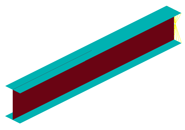
Figure 2.
Tip: Quickly import the model by dragging and
dropping the h3d file from a windows browser into the
HyperLife
modeling window.
Define the Fatigue Module
-
From the Setup tools, click the
SN tool.
The SN tool should be the default fatigue module selected. If it is not, click the arrow next to the fatigue module icon to display a list of available options.
Figure 3.The SN dialog opens. -
Define the SN configuration parameters.
- Select Multi Axial as the method.
- Select MPA for the FE model units.
- Enter a value of 0.5 for the certainty of survival.
- Select GOODMAN for the Tension Damage Model.
- Select NONE for the Shear Damage Model.
- Select Worst for the layer selection.
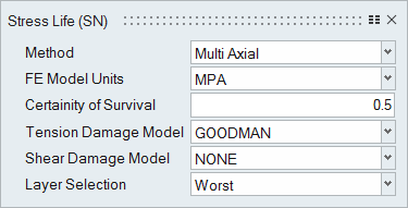
Figure 4.
Assign Materials
-
From the Setup tools, click the
Material tool.

Figure 5.The Assign Material dialog opens. -
Create a new material.
-
Click
 to create a new material.
-
Accept all other default settings then click Plot &
Save.
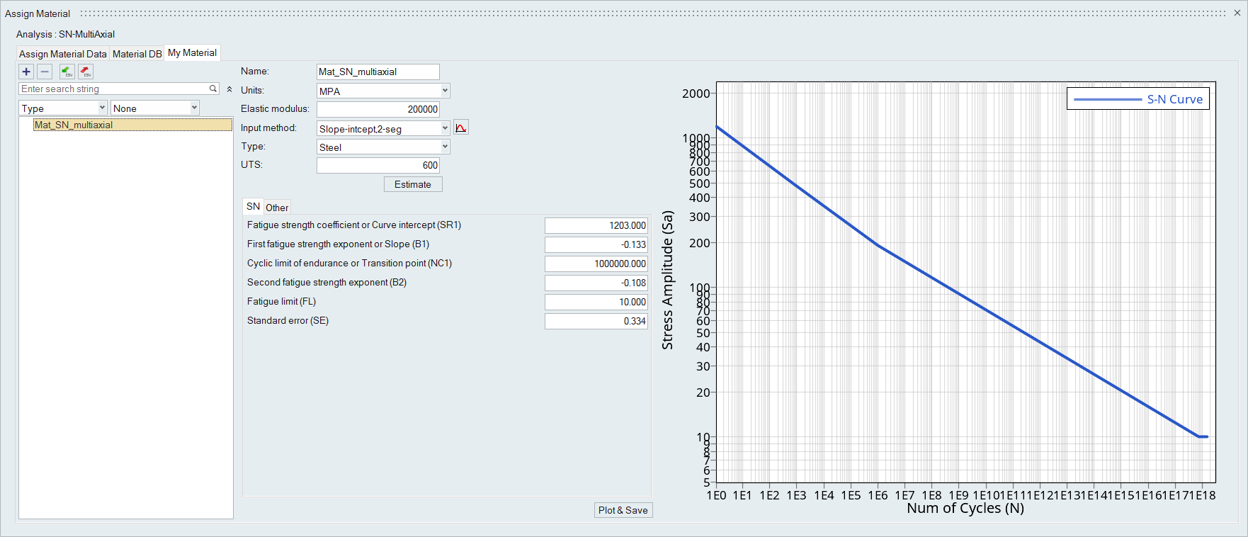
Figure 6.
-
Click
-
Return to the Assign Material Data tab and select
Mat_SN_multiaxial from the Material drop-down menu
for both Flange and Web.
The Material list is populated with the materials selected from Material Database and My Material.
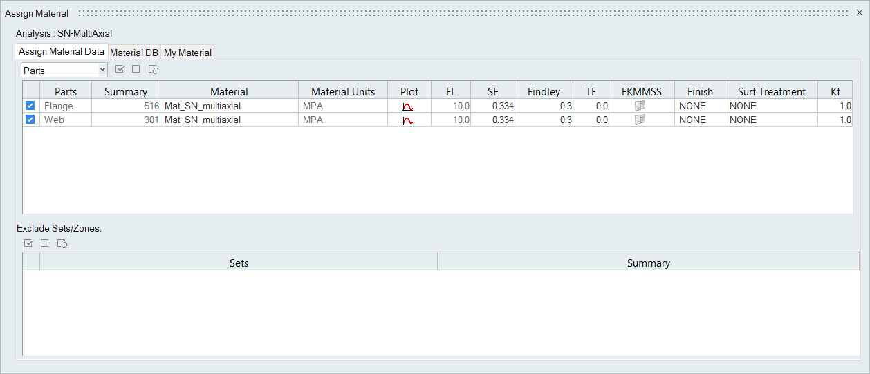
Figure 7.
Assign Load Histories
-
From the Setup tools, click the
Load Map tool.

Figure 8.The Load Map dialog opens. -
Click
 and browse for
load1.csv.
and browse for
load1.csv.
-
Click to add the load case.
- Optional:
Click
 to view a plot of the loads.
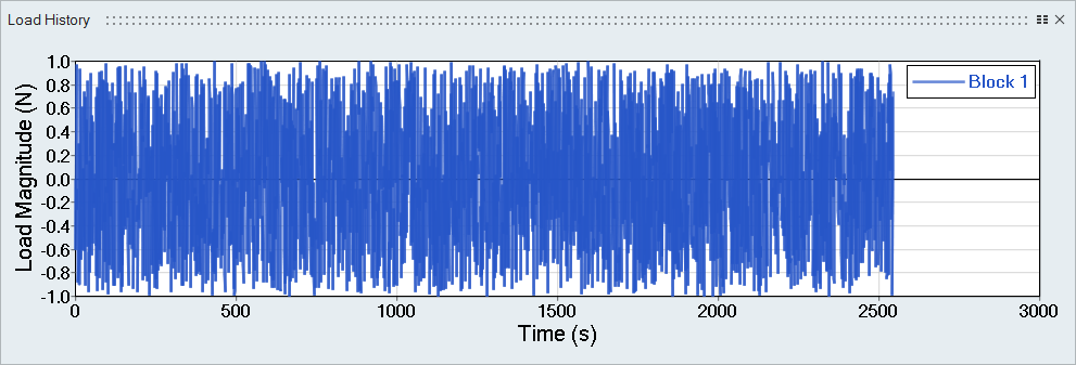
Figure 9. Load 1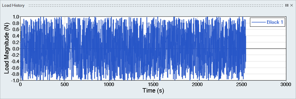
Figure 10. Load 2Tip: Expand the width of the dialog to view a clearer picture of the plot. -
Select both the Block 1 channel under load1 and
Subcase 1, then click
to create the first event.
-
Set the Scale to 8.0 for subcase 2.
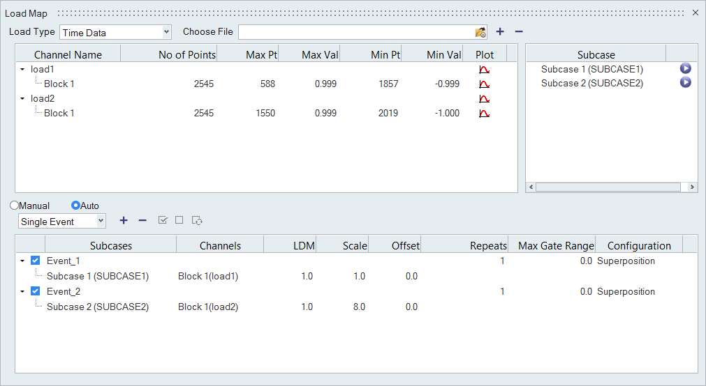
Figure 11.
Evaluate and View Results
-
From the Evaluate tool group, click the Run Analysis tool.

Figure 12.The Evaluate dialog opens.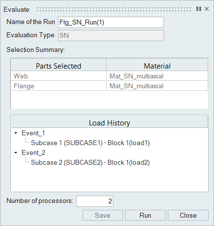
Figure 13. -
Click Run.
Result files are saved to the home directory and the Run History dialog opens.
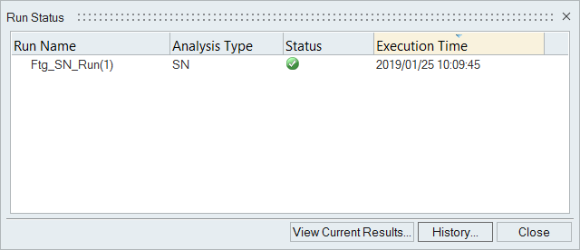
Figure 14. -
Use the Results Explorer to
visualize various types of results.
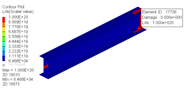
Figure 15.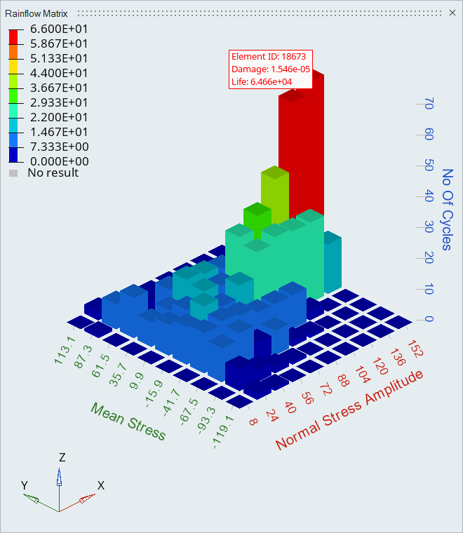
Figure 16.The life expectancy for the worst element is 64,660 cycles.