Stress-Life (S-N) Approach

During Transient Fatigue Analysis, the load-time history input is not required, as it is calculated internally during transient analysis.

This example will detail a Stress-Life fatigue calculation for a transient subcase. Transient Fatigue Analysis is currently supported for SN (uniaxial and multiaxial) and EN (uniaxial and multiaxial)

In this tutorial you will:

Import a model to HyperLife
Select the SN module and define its required parameters
Create and assign materials
Create an event
Evaluate and view results

Prior to running through this tutorial, copy Models-h3d.zip from <HyperWorks_installation_directory>\tutorials\hl to a local directory. Extract Bracket-SN-Transient.h3d from Models-h3d.zip..

Import the Model

From the Home tools, Files tool group, click the Open Model tool.

Figure 1.
From the Load model and result dialog, browse and select Bracket-SN-Transient.h3d for the model file.
The Load result field is automatically populated. For this tutorial, the same file is used for both the model and the result.
Click Apply.

Figure 2.

Tip: Quickly import the model by dragging and dropping the h3d file from a windows browser into the HyperLife modeling window.

Define the Fatigue Module

From the Setup tools, click the SN tool.
The SN tool should be the default fatigue module selected. If it is not, click the arrow next to the fatigue module icon to display a list of available options.

Figure 3.

The SN dialog opens.
Define the SN configuration parameters.
1. Select Uni Axial as the method.
2. Select MPA for the FE model units.
3. Select Signed von for the stress combination.
4. Enter a value of 0.6 for the certainty of survival.
5. Select GOODMAN for the mean stress connection.
6. Select Worst for the layer selection.
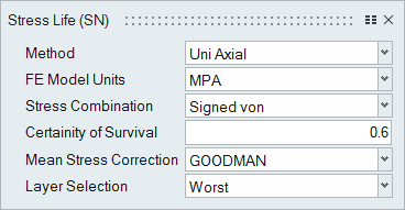
Figure 4.
Exit the dialog.

Assign Materials

From the Setup tool group, click the Material tool.

Figure 5.

The Assign Material dialog opens.
Activate the checkbox next to new_bracket.
Create a new material.
1. Click the My Material tab.
2. Click to create a new material.
3. Set the Elastic modulus to 200000.
4. Change the Input method to Slope-intcept,2-seg.
5. Set UTS to 2000.
6. In the SN tab, set the Fatigue strength coefficient or Curve intercept (SR1) to 1040.
7. Set the First fatigue strength exponent or Slope (B1) to -0.231.
8. Set the Cyclic limit of endurance or Transition point (NC1) to 600000.
9. Set the Second fatigue strength exponent (B2) to -0.110.
10. Set the Fatigue limit to 10.
11. Set the Standard error value to 0.01.
12. Click the Other tab and set Yield Strength to 1800.
13. Click Plot & Save.
  
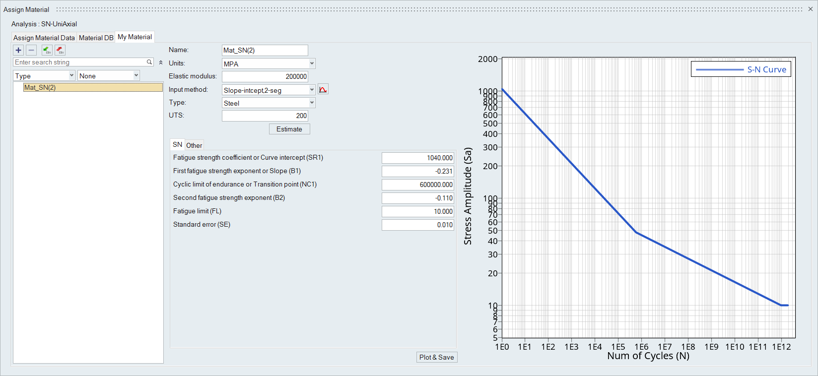
  Figure 6.
Right-click on Mat_SN("n") and select Add to Assign Material List.
Return to the Assign Material tab and select Mat_SN("n") from the Material drop-down menu for new_bracket.
The Material list is populated with the materials selected from Material Database and My Material.
Set Finish to POLISH, Surf Treatment to NITRIDED, and Kf to 1.3.

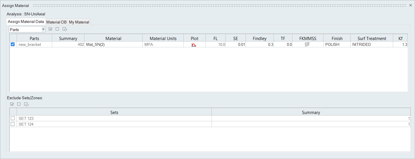
Figure 7.
Exit the dialog.

Assign Load Histories

From the Setup tool group, click the Load Map tool.

Figure 8.

The Load Map dialog opens.
From the Load Type menu, select Transient Response.
Since this is a transient fatigue analysis, a load history is not required.
Select Subcase 1 (transient).
On the bottom half of the dialog, set the radio button to Auto for event creation and click to create an Event_1 header.
Subcase 1 is listed under the event.
Activate the Event_1 checkbox.

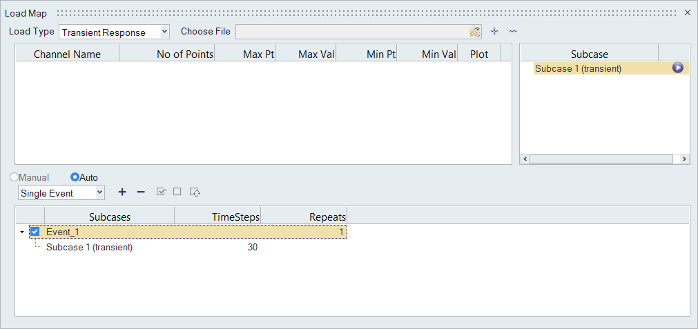
Figure 9.
Exit the dialog.

Evaluate and View Results

From the Evaluate tool group, click the Run Analysis tool.

Figure 10.

The Evaluate dialog opens.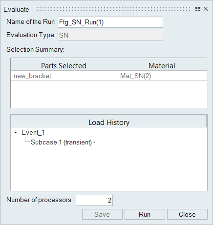

Figure 11.
Optional: Enter a name for the run.
Click Run.
Result files are saved to the home directory and the Run History dialog opens.

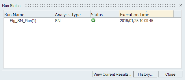
Figure 12.
Once the run is complete, click View Current Results.
Use the Results Explorer to visualize various types of results.

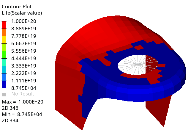
Figure 13.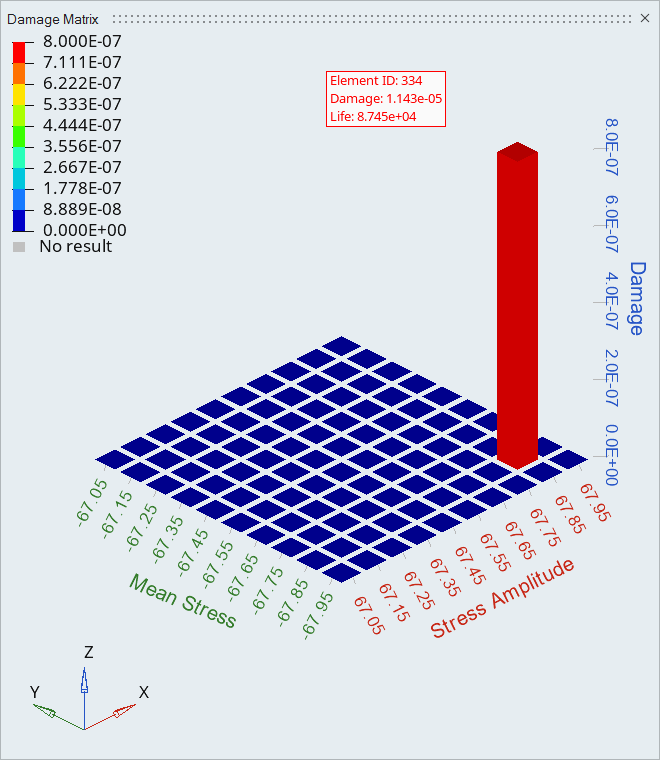

Figure 14.