Acoustic Infinite Elements
Acoustic modeling in finite and semi-infinite domains is essential in the prediction of quantities such as external and radiated noise in vibro-acoustic problems. Infinite elements are a popular way of modeling these domains. Acoustic Infinite Elements are supported for both Direct and Modal Frequency Response analyses.
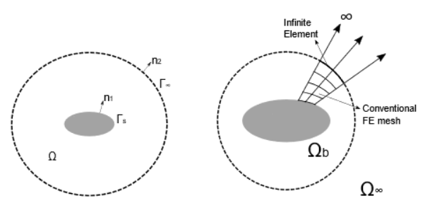
Figure 1. Acoustic Problem on an Infinite Domain
Implementation
Considering the domain in the figure above, the region surrounding the structure (shaded area) is modeled using a conventional fluid FE mesh, and the far field is modeled using infinite elements defined on a 2D interface between the finite and infinite (unbounded) domains.
- Wave number
- Circular frequency
- Speed of sound
- Unit normal to the surface of the fluid elements
- Unit normal to the surface of the "infinite boundary" (sufficiently far away from the structure)
- Pressure
- Fluid density
- Displacement of the structural boundary in the direction
Input/Output
Input
- Fluid material properties (bulk modulus, speed of sound, fluid density) can be specified for the fluid elements on the MAT10 Bulk Data Entry.
- Pole location (origin of the acoustic disturbance). Pole is the center of acoustic disturbance. This can be defined on the PACINF Bulk Data Entry via the XP, YP, ZP coordinates.
- The nodes defining the interface between the infinite and semi-infinite domain. This is defined as the Infinite elements (currently 3-noded CACINF3 and 4-noded CACINF4 elements are supported).
- The radial interpolation order can be specified via the RIO field on the PACINF entry.
Modeling
- A minimum of 1 layer of Fluid elements should be defined on the surface of the structural domain of interest.
- The Infinite elements (CACINF3 and CACINF4) should only be defined on the topmost surface of the Fluid elements.
- See Output for more information.
- Infinite Elements modeling practice can be typically recommended as:
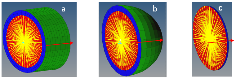
Figure 2. Modeling Practices for Infinite Elements . (Green elements: Infinite Elements, Red color arrow is direction of receiver, Blue Elements: Acoustic elements)Correct Modeling PracticesIncorrect Modeling Practices:- In Figure 2(c), infinite elements are the skin on the fluid acoustic elements covering one of the sides (front side) in the direction of the receiver.
- Normals of infinite elements should always point away from the pole.
- Sound pressure can be measured on the receiver grid points. For visualization of the sound pressure contour, the receiver elements should be PLOTEL elements.
- Source is generally a structure which is excited by a load, which also can be fluid grid with SLOAD.
Output
Currently only Pressure output is supported for any grid points in the acoustic domain using Infinite Elements. The Pressure output can be requested using the DISPLACEMENT I/O Options Entry. Pressure can be requested for grid points belonging to the fluid domain of the model at external microphone locations which can be specified as GRID point sets.