ACU-T: 3201 Greenhouse
Daytime Climate Simulation – Solar Radiation and Thermal Shell
This tutorial provides the instructions for setting up, solving and viewing results for a
steady simulation of air flow through a greenhouse using solar and enclosure radiation along
with thermal shell and porous media. In this simulation, AcuSolve is used
to compute the temperature and solar flux distribution due solar radiation incident on the
roof which is modeled as a thermal shell. This tutorial is designed to introduce you to a
number of modeling concepts necessary to perform simulations that use thermal shells and
solar radiation.
Prior to running through this tutorial, copy
AcuConsole_tutorial_inputs.zip from
<AcuSolve_installation_directory>\model_files\tutorials\AcuSolve
to a local directory. ExtractGreenhouse_Solar.x_t, solar_flux.dat and
Greenhouse_Enclosure_Night.acsfrom AcuConsole_tutorial_inputs.zip.
Analyze the Problem
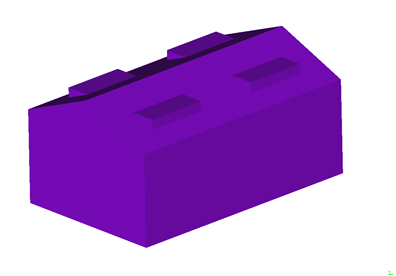
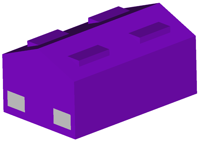
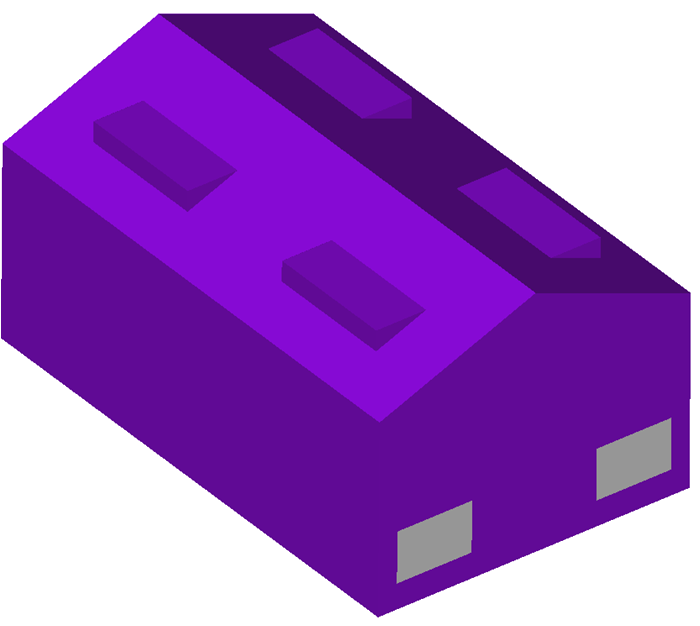
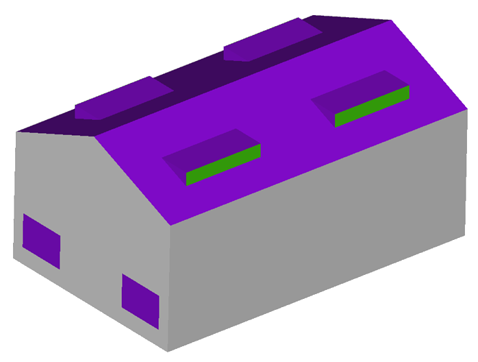
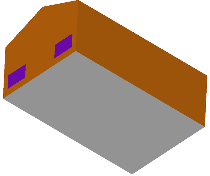
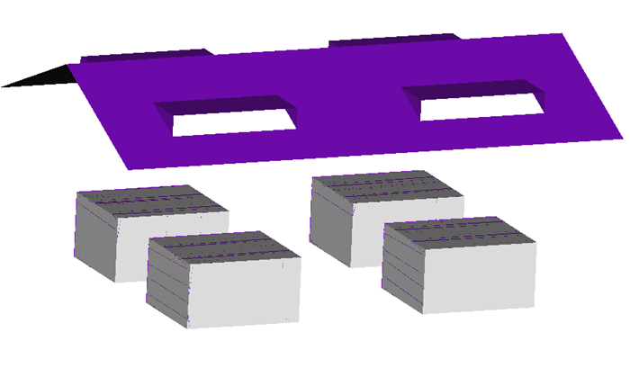
The problem to be addressed in this tutorial is shown schematically in Figure 1. It consists of a low cost
gable type greenhouse with tomato plants modeled as porous media, and four inlets and outlet
vents. The roof of the greenhouse is modeled as a thermal shell with three layers in order to
account for heat transfer due to its thickness. The fluid enters through the inlet vents, passes
through the tomato plants, and then exits the greenhouse through the outlet vents located on the
roof.
Greenhouses are high-tech structures dedicated to the horticultural needs of plants,
particularly flowers, vegetables and fruits. Environmental properties such as temperature, light
exposure, irrigation, fertilization, humidity and ventilation can be precisely controlled for
optimal crop growth.
The geometric characteristics of the greenhouse are as follows:
Total Length: 4 m
Total Width: 2 m
Eaves Height: 1.5 m
Ridge Height: 2 m
Inlet Vents (4): 0.6 m length X 0.4 m height
Outlet Vents (4): 1m length X 0.4 m height
Figure 1. Schematic of Greenhouse
Air enters the inlet vent at an average speed of 1.8 m/s and temperature 303 K which is
considered the temperature of ambient air around the greenhouse. The outlet vent is considered a
constant pressure (p = patm) outlet boundary.
The fluid in this problem is air, which has the following material properties:
Density (ρ): 1.225 kg/m3
Viscosity (µ): 1.781 X 10⁻⁵ kg/m-s
Specific Heat (Cp): 1005 J/kg-K
Conductivity (k): 0.0251 W/m-K
The density variation will be calculated according to the Boussinesq model in order to take
into account the natural convection effects.
The simulation will be set up to model steady state, turbulent flow in order to determine the
climate distribution inside the greenhouse at day time, due to the incident solar radiation.
Analyze of the Solar Radiation Properties of the Model
The incident solar radiation is computed using the acuSflux script provided with the
installation. The location is selected as Sunnyvale California, USA at latitude 37.3688° N
and longitude 122.0363° W. The date is selected as 30th August 2016. The time of the day is
taken as 10:30 am in the morning.
The solar radiation is modeled by adding the solar fluxes to the thermal energy equation
computed using a ray trace algorithm. The ray trace algorithm uses the Monte Carlo method to
compute exchange factors and the solar heat flux on every surface.
The interaction of a solar ray photon with a surface may occur in five different ways:
Specular transmission : Photon passes straight through a surface with no
change of direction.
Diffuse transmission : Photon penetrates the surface, but its outgoing energy
is uniformly distributed in solid angle over the hemisphere, weighted by projected
surface area.
Specular reflection : angle of reflection is equal to the angle of
incidence.
Diffuse reflections : similar to diffuse transmission, except the hemisphere
over which the outgoing energy is distributed is on the same side of the surface as the
incident photon.
Absorption : Photon may be absorbed by the surface.
These five interactions are associated with five surface properties that together obey the
following constraint:
For computation purposes all of the surfaces are assumed to be gray bodies, that is,
emissivity and absorption are assumed to be independent of wavelength. Further from
Kirchhoff’s law of radiation absorptivity is assumed to be equal to the emissivity of the
material.
The cover material on the roof of the greenhouse is semi-transparent and the plants, ground
and walls are diffusively radiating opaque surfaces.
The solar radiation/optical properties of the materials are listed below:
Cover:
Plants:
Ground:
Walls:
Analyze of the Thermal Shell
Thermal shells are used to model the energy equation in solid materials where the thinness
of the geometry makes it inconvenient to use it as solid. A solid or shell element set
solves only the temperature and mesh displacement equations, while all other equations, such
as flow, turbulence, and species, are ignored.
Geometrically, the shell is infinitely thin, so that the pairs of nodes in an element that
are on opposite sides of the shell have the same coordinates. The shell medium supports only
wedges and bricks.
For a single layer thermal shell the complete 3D heat transfer equation is solved
considering the complete volume element of thickness specified. For multiple layer thermal
shell, between the two sides of the shell, the element is divided up into a number of
layers. Each layer is assigned a material model and a thickness and a one dimensional heat
equation is solved through the shell thickness.
The roof of the greenhouse is modeled as a thermal shell with four layers each of thickness
0.25 cm.
The material model of the thermal shell has the following properties:
In addition to setting appropriate conditions for the simulation, it is important to
generate a mesh that will be sufficiently refined to provide good results. For this problem
the global mesh size is set to provide at least 33 elements along the biggest dimensions of
the greenhouse, the length.
Note that higher mesh densities are required where velocity, pressure, and eddy viscosity
gradients are larger. Local mesh refinements are used for the volume region containing the
porous media and the inlet and outlet surfaces. Proper boundary layer parameters need to be
set to keep the y+ near the wall surface to a reasonable level. The mesh density used in
this tutorial is coarse and is intended to illustrate the process of setting up the model
and to retain a reasonable run time. A significantly higher mesh density is needed to
achieve a grid converged solution.
Once a solution is calculated, the flow properties of interest are the temperature
distribution on the ground and roof and the solar flux on the roof of the greenhouse.
Define the Simulation Parameters
Start AcuConsole and Create the Simulation Database
In this tutorial, you will begin by opening an existing database, modifying and
adding the geometry-independent settings, replacing the geometry, creating
additional groups, setting group parameters, adding geometry components to groups,
and assigning mesh controls and boundary conditions to the groups. Next you will
generate a mesh and thermal shell with its associated properties. Then you will run
AcuSolve to compute the steady state solution.
Finally, you will visualize the results using AcuFieldView.
In the next steps you will start AcuConsole open and
rename the database for storage of the simulation settings.
Start AcuConsole from the Windows Start menu by clicking Start > All Programs > Altair HyperWorks <version> > AcuSolve > AcuConsole.
From the File menu, click Open to open the
Open data base dialog.
Note: You can also open the dialog by clicking on the
toolbar.
Open the Greenhouse_Enclosure_Night.acs file.
Browse to the location that you would like to use as your working
directory.
This directory is where all files related to the simulation will
be stored. The AcuConsole database file
(.acs) is stored in
this directory. Once the mesh and solution are created, additional files and
directories will be created within this directory.
Create a new folder named Greenhouse_Solar_Day and open
this folder.
Enter Greenhouse_Solar_Day as the File name for the
database.
Note: In order for other applications to be able to read the
files written by AcuConsole, the database
path and name should not include spaces.
Save the database to create a backup
of your settings.
Set General Simulation Parameters
In next steps you will set the parameters that apply
globally to the simulation. To simplify this task, you will use the BAS filter in
the Data Tree Manager. This filter limits the options in the
Data Tree to show only the basic settings.
The physical models that you define for this tutorial correspond to steady state,
turbulent flow.
Click BAS in the Data Tree Manager to switch to basic view in the Data Tree.
Figure 2.
Double-click the GlobalData Tree item to expand it.
Tip: You can also expand a tree item
by clicking
next to the item name. Figure 3.
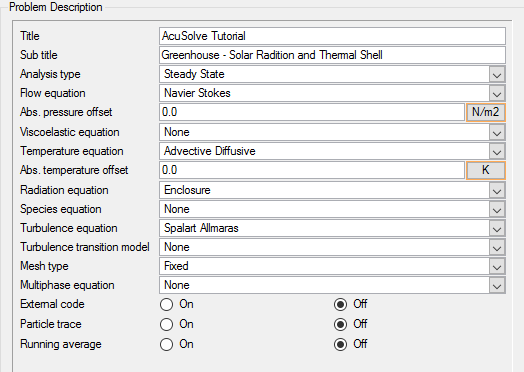
Double-click Problem
Description to open the Problem
Description detail panel.
Check that AcuSolve Tutorial is the Title.
Enter Greenhouse - Solar Radiation and Thermal Shell as
the Sub title.
Accept the default Analysis type of Steady State.
Check that the Turbulence equation is set to Spalart
Allmaras.
Check that the Temperature equation is set to Advective
Diffusive.
Check that the Radiation equation is set to
Enclosure.
Accept the default Mesh type of Fixed.
Figure 4.
Tip: You may need to widen the detail panel from the default size by
dragging the right edge of the panel frame.
Set Solution Strategy Parameters
In the next steps you will set the parameters that control the behavior of AcuSolve as it progresses during the solution.
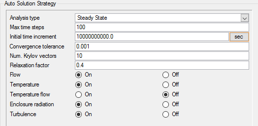
Double-click Auto Solution
Strategy to open the Auto Solution
Strategy detail panel.
Check that the Analysis type is set to
Steady State.
Ensure that Max time steps is set to
100.
Check that the Convergence tolerance is set to 0.001
seconds.
Set the Relaxation factor to 0.4.
The relaxation factor is used to improve convergence of the solution.
Typically a value between 0.2 and 0.4 provides a good balance between achieving
a smooth progression of the solution and the extra compute time needed to reach
convergence. Higher relaxation factors cause AcuSolve to take more time steps to reach a steady state solution. A high relaxation
factor is sometimes necessary in order to achieve convergence for very complex
applications. Figure 5.
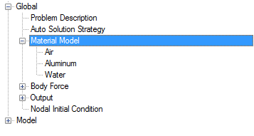
Set Material Model Properties
AcuConsole has three pre-defined materials, Air,
Aluminum and Water. You will need to modify the material properties of Aluminum and
create a new material model which would model the properties of cover material for
defining the thermal shell in the later steps.
In the next steps you will modify the
density of aluminum. Additionally, you will create a new material model named
Cover_Shell and assign the material properties associated with it.
Double-click Material Model
in the Data Tree to expand it.
Figure 6.
Right-click Aluminum in the
Data Tree and select
Duplicate to make a copy of the Aluminum material
model.
Right-click Copy of Aluminum in the Data Tree and select Rename. Enter
Cover_Shell as the new name.
Double-click Cover_Shell to open the detail panel.
Check that the Material type for Cover_Shell is Solid.
The default material type for any new material created in AcuConsole is Fluid.
Click the Density tab.
The density of cover is 930.0 kg/m3.
Click the Specific Heat tab. The specific heat of plants
is 2000 J/kg-K.
Click the Conductivity tab. The conductivity of cover is
0.35 W/m-K.
Save the database to create a backup
of your settings. This can be achieved with any of the following
methods.
Click the File menu, then click
Save.
Click on
the toolbar.
Click Ctrl+S.
Note: Changes made in AcuConsole are saved into
the database file (.acs) as they are made. A save operation copies the database to
a backup file, which can be used to reload the database from that saved
state in the event that you do not want to commit future changes.
Create New Solar Radiation Models
The solar radiation models command specifies an ideal grey-surface solar radiation
model to calculate the solar heat flux. AcuConsole has a
predefined solar radiation model for a black body. You will need to create
additional solar radiation models for the roof, greenhouse walls, plants and the
floor surface covered by soil.
In the next steps you will create new solar radiation models and the assign the
values associated with them.
Click RAD in the Data Tree Manager
to filter all but the radiation settings in the Data Tree.
Double-click Solar Radiation Model in the Data Tree to expand it.
Right-click Solar Radiation Model in the Data Tree and select New to make a new
solar radiation model.
A new solar radiation model will be created with the name Solar
Radiation Model 1.
Right-click Solar Radiation Model 1 and select
Rename.
Enter Cover as the new name.
Double-click Cover to open the detail panel.
Check that Type is set as Constant for all the parameters.
Enter the values for the cover material as shown in the figure below.
Figure 7. Cover Solar Radiation Detail Panel
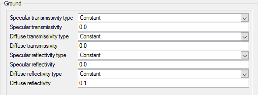
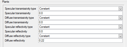
Similarly create three more solar radiation models named: Ground, Plants and
Walls and set their solar radiation values as shown below.
Figure 8. Ground Solar Radiation Detail Panel Figure 9. Plants Solar Radiation Detail Panel Figure 10. Walls Solar Radiation Detail Panel
Define the Solar Radiation Parameters
The solar radiation parameters command specifies the global parameters for solar
radiation heat flux. AcuConsole has a predefined solar
radiation flux of -1352.0 W/m2 in the –Z direction.
The value would be read from the file solar_flux.dat generated
by the acuSflux script.
Double-click Solar Radiation Parameters in the Data Tree to expand it.
Click Open Array next to Curve fit values.
In the Array Editor, click Read and
open the file solar_flux.dat.
The solar flux is read and stored into the respective columns in the
Array Editor.
Click OK to close the dialog.
Tip: To generate the solar_flux.dat file,
execute the following command from the command
line:
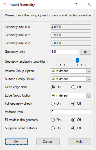
You will import the geometry in the next
part of this tutorial. You will need to know the location ofGreenhouse_Solar.x_tin order to complete these steps. This file contains
information about the geometry in ParasolidASCII format.
Click File > Import.
Browse to the directory containing Greenhouse_Solar.x_t.
Change the file name filter to Parasolid File (*.x_t *.xmt *X_T
…).
Select Greenhouse_Solar.x_t and click
Open to open the Import Geometry
dialog.
Figure 11.
For this tutorial, the default values for the Import
Geometry dialog are used to load the geometry. If you have previously
used AcuConsole, be sure that any settings that you
might have altered are manually changed to match the default values shown in the
figure. With the default settings, volumes from the CAD model are added to a default
volume group. Surfaces from the CAD model are added to a default surface group. You
will work with groups later in this tutorial to create new groups, set flow
parameters, add geometric components, and set meshing parameters.
Click Ok to complete the geometry import.
Figure 12.
The color of objects shown in the modeling window in this tutorial and those displayed on your screen may differ. The default color
scheme in AcuConsole is "random," in which colors are
randomly assigned to groups as they are created. In addition, this tutorial was
developed on Windows. If you are running this tutorial on a different operating system,
you may notice a slight difference between the images displayed on your screen and the
images shown in the tutorial.
Apply Volume Parameters
Volume groups are containers used for storing information about a volume region. This
information includes the list of geometric volumes associated with the container, as
well as attributes such as material models and mesh size information.
When the geometry was imported into AcuConsole, all
volumes were placed into the "default" volume container.
In the next steps you will assign the volumes to existing volume groups.
Click BAS in the Data Tree Manager to switch to basic view in the Data Tree.
Expand the ModelData Tree item.
Expand Volumes. Toggle the display of the default
volume container by clicking
and next to the volume name.
Note: You may not see any change when toggling the display if
Surfaces are being displayed, as surfaces and
volumes may overlap.
Add the volume to the Greenhouse_Main group.
Right-click Greenhouse_Main > Add to.
Click on the greenhouse.
At this point, the greenhouse should be highlighted in the color
gray. Figure 13.
Add the volume to Greenhouse_Plants groups.
Right-click Greenhouse_Plants and select Add
to.
Click on the plant.
At this point, the greenhouse plants should be highlighted in the color
gray. Figure 14.
Figure 15.
Right-click on the default volume group and select
delete.
Check that the material model for the volume Greenhouse_Main is set to
Air.
Expand the Greenhouse_Main volume.
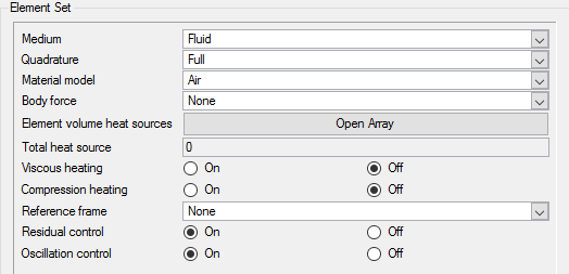
Double-click Element Set under Greenhouse_Main
to open the Element Set detail panel.
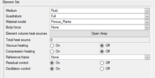
Check that the Material model is set as Air.
Figure 16.
Check that the material model for the volume Greenhouse_Plants is set to
Porous_Plants.
Expand the Greenhouse_Plants volume.
Double-click Element Set under Greenhouse_Main
to open the Element Set detail panel.
Check that the Material model is set as Porous_Plants.
Figure 17.
Set Surface Meshing Parameters
Surface groups are containers used for storing information about a surface. This
information includes the list of geometric surfaces associated with the container,
as well as attributes such as boundary conditions, surface outputs, and mesh sizing
information.
When the geometry was replaced into AcuConsole, all
surfaces are placed in the surface container named "default" and the existing
surface groups becoming empty.
In the next steps you will define surface groups, assign the appropriate settings for
the different characteristics of the problem, and add surfaces to the group
containers.
Inlets_1
Inlets_2
Outlet
Greenhouse_Walls
Plant_Cover
Roof
Ground
Set Parameters for the Inlet
In the next steps you will create a copy of surface group Inlet, rename them to
Inlets_1 and Inlets_2, assign the appropriate settings, and add the inlets from the
geometry to the surface groups.
Create a copy of the Inlet surface group.
In the Data Tree, right-click on
Inlet and select
Duplicate.
Right-click Inlet and rename it to
Inlets_1.
Right-click Copy of Inlet and rename it to
Inlets_2.
Expand the Inlets_1 surface in the Data Tree.
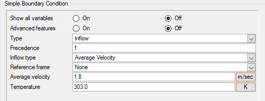
Double-click Simple Boundary Condition under Inlets_1 to
open the Simple Boundary Condition detail panel.
Change the Type to Inflow.
Change the Average velocity value to 1.8 m/s.
Change the Temperature to 303.0 k.
Figure 18.
Click RAD in the Data Tree Manager.
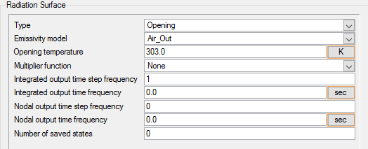
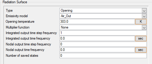
Under Inlets_1, double-click the Radiation Surface
check box to activate and open the Radiation Surface detail
panel.
Check that the Type is set to Opening.
Check that the Emissivity model is set to Air_Out.
Set the Opening temperature value to 303 K.
Figure 19.
Add a geometry surface to the Inlet group.
Right-click Inlet > Add to.
Click on the inlet face.
At this point, the inlet should be highlighted by the color gray. If
it is difficult to find the inlet surface, change the display type to
outline to see where the inlet is located. Figure 20.
Click Done to add this geometry surface to the
Inlet surface group.
You can also use the middle mouse button to complete the
addition of geometry components to a group.
Propagate the settings for Simple Boundary Condition and Radiation Surface to
the Inlets_2 surface group.
Note: You may need to switch between BAS and RAD in the Data Tree Manager or display all the attributes by selecting
the ALL filter.
Under Inlets_1, right-click on Simple Boundary
Condition and select
Propagate.
The Propagate dialog appears.
Select Inlets_2 from the list, and click
Propagate.
Under Inlets_1, right-click on Radiation Surface and select
Propagate.
Select Inlets_2 from the list, and click
Propagate.
Add a geometry surface to the Inlets_2 group.
Right-click Inlets_2 and click Add
to.
Click on the inlet faces on the +X sides of the geometry.
Figure 21.
At this point, the inlets should be highlighted by grey color. If it
is difficult to find the inlet surfaces, change the display type to
outline to see where the inlets are located.
Set Parameters for the Outlet
In the next steps you will assign the appropriate settings, and add the outlet from
the geometry to the surface group
Click BAS in the Data Tree Manager to switch to basic view in the Data Tree.
Expand the Outlet surface group in the Data Tree.
Double-click Simple Boundary Condition to open the
detail panel.
Check that the Type is set to Outflow.
Click RAD in the Data Tree Manager.
Under Outlet, activate the Radiation Surface check box
and double-click it to open the detail panel.
Check that the Type is set to Opening.
Check that the Emissivity model is set to Air_Out.
Change the Opening temperature value to 303 K.
Figure 22.
Add a geometry surface to the Outlet surface container.
Right-click Outlet > Add to.
Click the outlet face.
At this point, the outlet should be highlighted by the color gray. Figure 23.
Click Done to associate this geometry surface
with the surface settings of the Outlet group.
Set Parameters for the Greenhouse_Walls
In the next steps you will define a surface group for the walls, assign the
appropriate settings and add the faces from the geometry to the surface group.
Click BAS in the Data Tree Manager to switch to basic view in the Data Tree.
Expand the Greenhouse_Walls surface in the Data Tree.
Under Greenhouse_Walls, double-click Simple Boundary
Condition and check that the Type is set to
Wall.
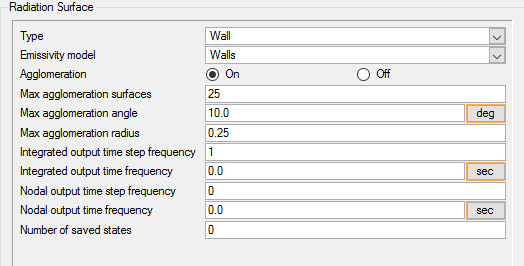
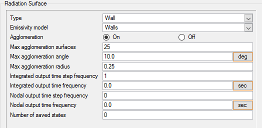
Click RAD in the Data Tree Manager.
Check that the Type is set to Wall.
Check that the Emissivity model is set to Walls.
Under Greenhouse_Walls, activate the Radiation Surface
to open the detail panel.
Figure 24.
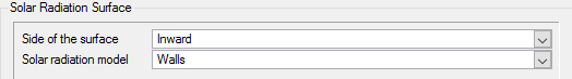
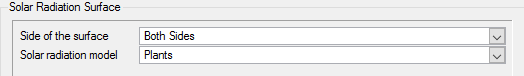
In the Data Tree, click the Solar Radiation Surface
check box to activate and open the detail panel.
For Side of Surface, select Inward.
For Solar Radiation model, select Walls.
Figure 25.
Add geometric faces to this group.
Right-click Greenhouse_Walls > Add to.
Select all of the wall surfaces.
At this point, the wall surfaces should be highlighted in gray. Figure 26.
Click Done to associate this geometry surface
with the Greenhouse_Walls surface container.
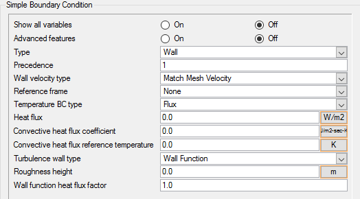
Set Parameters for the Ground
In the next steps you will define a surface group for the ground, assign the
appropriate settings and add the faces from the geometry to the surface group.
Click BAS in the Data Tree Manager to switch to basic view in the Data Tree.
Expand the Ground surface.
Double-click Simple Boundary Condition to open the
detail panel.
Check that the Type is set to Wall.
Set the Temperature BC type to Flux.
The default value of 0 is used for the Heat Flux for the ground. Figure 27.
Click RAD in the Data Tree Manager.
Under Ground, activate the Radiation Surface to open the
detail panel.
Check that the Type is set to Wall.
Check that the Emissivity model is set to Ground.
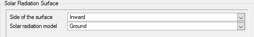
In the Data Tree, click the Solar Radiation Surface
check box to activate and open the detail panel.
For Side of Surface, select Inward.
For Solar Radiation model, select Ground.
Figure 28.
Add geometric faces to this group.
Right-click Ground > Add to.
Select the ground surface.
At this point, the ground surface should be highlighted by the color
gray. Figure 29.
Click Done to add this geometry surface to the
Ground surface group.
Set Parameters for Plant Cover Surfaces
In the next steps you will define surface groups for the plant cover, assign the
appropriate settings and add the plant cover surfaces from the geometry to the
surface group.
Turn off the visibility for the Ground, Walls, Inlets and Outlet
surfaces.
Rename the surface Plant_Cover_Upstream to
Plant_Cover.
Add the geometry surface to the Plant_Cover surface group.
Right-click Plant_Cover > Add to.
Click all the plant surfaces.
If it is difficult to find the surface, turn on the visibility for the
volume group and set the display type to Outline. Figure 30.
At this point, the Plant_Cover surface should be highlighted in
gray.
Click Done to add this geometry surface to the
Plant_Cover surface group.
Turn off the display for the surface.
There are two sets of surfaces for the plant surfaces which belong to
different volume sets. In this case they can be moved into the same
surface group.
Right-click Plant_Cover > Add to.
Select the remaining Plant_Cover surfaces.
Click Done to associate this geometry surface
with the surface settings of the Plant_Cover group.
Note that no boundary conditions are applied to this surface at this
point. The grouping operation was performed to identify that these
surfaces are internal and that flow will be allowed to pass through them
freely. These surfaces can still be used for output purposes,
however.
Click RAD in the Data Tree Manager.
Under Plant_Cover, activate the Radiation Surface to
open the detail panel.
Check that the Type is set to Wall.
Check that the Emissivity model is set to Plants.
In the Data Tree, click the Solar Radiation Surface
check box to activate and open the detail panel.
For Side of Surface, select Both Sides.
For Solar Radiation model, select Plants.
Figure 31.
Set Parameters for the Roof Surfaces
In the next steps you will define surface groups for the roof, assign the appropriate
settings and add the roof surface from the geometry to the surface group.
Turn off the visibility for the Plant_Cover surfaces.
Rename the surface Plant_Cover_Downstream to Roof.
Under Roof, double-click Simple Boundary Condition and
check that the Type is set to Wall.
Click RAD in the Data Tree Manager.
Under Roof, activate the Radiation Surface to open the
detail panel.
Check that the Type is set to Wall.
Set the Emissivity model to Walls.
Figure 32.
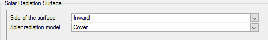
In the Data Tree, click the Solar Radiation
Surface check box to activate and open the detail panel.
For Side of Surface, select Inward.
For Solar Radiation model, select Cover.
Figure 33.
Add the geometry surface to the Roof group.
Right-click Roof > Add to.
Click the roof surfaces.
Click Done to add this geometry surface to the
Plant_Cover surface group.
Note: At this point, all remaining volume containers, including the default
container, should be empty.
Right-click on Surfaces and click
Purge to remove the empty volume containers.
Assign Mesh Controls
Set Global Meshing Attributes
Now that the flow characteristics have been set for the whole problem and for the
individual surfaces, attributes need to be added to make sure that a sufficiently
refined mesh is generated.
Global mesh controls apply to the whole model without being tied to any
geometric component of the model.
Zone mesh controls apply to a defined region of the model, but are not
associated with a particular geometric component.
Geometric mesh controls are applied to a specific geometric component. These
controls can be applied to volume groups, surface groups or edge groups.
In the next steps you will set global meshing attributes. In subsequent steps you
will set the volume and surface meshing attributes.
Click MSH in the Data Tree Manager to filter the
settings in the Data Tree to show only the controls
related to meshing.
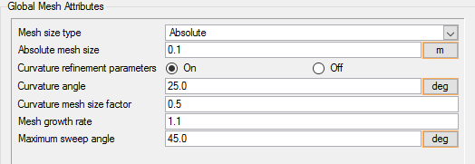
Double-click the GlobalData Tree item to expand it.
Double-click Global Mesh
Attributes to open the Global Mesh
Attributes detail panel.
Check that the Mesh size type to Absolute.
Enter 0.1 m for the Absolute mesh size.
This absolute mesh size is chosen to ensure that there are at least 33 mesh
elements on the inlet.
Set the Mesh growth rate to 1.1.
This option is used to control the rate at which the mesh transitions between
regions of different surface and volume size. By default, the mesher will
increase in size at a rate of approximately 2:1 between regions of adjacent
size within the mesh. By setting this option to a value between 1.0 and 2.0,
the mesh transition will be smoother across the size transitions.
Figure 34.
Set Volume Meshing Attributes
In the following steps you will set the meshing attributes that will allow for
localized control of the mesh size on the volume groups that you created earlier.
Specifically, you will set local meshing attributes that control the size of elements
inside the Greenhouse_Plants volume group.
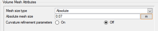
Expand the Model > Volume > Greenhouse_PlantsData Tree item.
Click the check box next to Volume Mesh Attributes to enable the settings and
open the Volume Mesh Attributes detail panel.
Enter 0.07 as the Absolute mesh size.
Figure 35.
Set Surface Meshing Parameters
In the following steps you will set the meshing attributes that will allow for
localized control of the mesh size on the surface groups that you created earlier.
Specifically, you will set local meshing attributes for inlet and outlet. You will
also set attributes that control the growth of boundary layer elements normal to the
surfaces of the greenhouse walls and ground.
Inlets_1
Inlets_2
Outlet
Greenhouse_Walls
Ground
Set Surface Meshing Parameters for the Inlet
In the following steps you will set meshing attributes that will allow for localized
control of the mesh size near the inlet.
Expand the Model > Surfaces > Inlets_2Data Tree item.
Click the check box next to Surface Mesh Attributes to enable the settings and
open the Surface Mesh Attributes detail panel.
Check that 0.05 is set as the Absolute mesh size.
Repeat for Inlets_1.
Set Surface Meshing Attributes for the Outlet
In the following steps you will set meshing attributes that will allow for localized
control of the mesh size near the outlet.
Expand the Model > Surfaces > OutletData Tree item.
Click the check box next to Surface Mesh Attributes to enable the settings and
open the Surface Mesh Attributes detail panel.
Enter 0.02 as the Absolute mesh size.
Set Surface Meshing Attributes for the Greenhouse Walls and Roof
In the following steps you will set meshing attributes that will allow for localized
control of the mesh size near the greenhouse walls. The mesh size on the wall will
be inherited from the global mesh size that was defined earlier. The settings that
follow will only control the growth of the boundary layer from the walls.
Expand the Model > Surfaces > Greenhouse_WallsData Tree item.
Click the check box next to Surface Mesh Attributes to enable the settings and
open the Surface Mesh Attributes detail panel.
Check that the Mesh size type is set to None.
This option indicates that the mesher will use the global meshing attributes
when creating the mesh on the surface of the walls.
Turn On the Boundary layer flag option.
This option allows you to define how the meshing should be handled in the
direction normal to the walls.
Check that the Boundary layer type is set to Full
Control.
Set Resolve to First Element Height.
Mesh elements for a boundary layer are grown in the normal direction from a
surface to allow efficient resolution of the steep gradients near no-slip walls.
The layers can be specified using a number of different options.
When Boundary
layer type is set to Full Control and the First Layer Height is resolved,
the Total layer height, Number of layers and the Growth rate are specified.
Boundary layer elements will be grown until the mesh size of the top layer
matches the mesh size of the volume into which the boundary layer elements
are grown.
Enter 0.1 m for the Total layer height.
Enter 1.1 for the Growth rate.
Enter 4 for the Number of layers.
Figure 36.
Propagate the Surface Mesh Attributes to the Roof surface.
Set Surface Meshing Parameters for the Ground
In the following steps you will set meshing attributes that will allow for localized
control of the mesh size near the fan blades.
Expand the Model > Surfaces > GroundData Tree item.
Click the check box next to Surface Mesh Attributes to enable the settings and
open the Surface Mesh Attributes detail panel.
Check that the Mesh size type is set to None.
Check that the Boundary layer flag option is turned on.
Set the Boundary layer type to Full Control.
Set Resolve to First Element Height.
Enter 0.08 m for the Total layer height.
Enter 1.1 for the Growth rate.
Enter 4 for the Number of layers.
Figure 37.
Save the database to create a backup
of your settings.
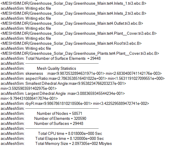
Generate the Mesh
In the next steps you will generate the mesh that will be used when computing a
solution for the problem.
Click
on the toolbar to open the Launch AcuMeshSim
dialog.
Click Ok to begin meshing.
During meshing an AcuTail dialog will open.
Meshing progress is reported in this dialog. A summary of the meshing process
indicates that the mesh generation has finished. Figure 38.
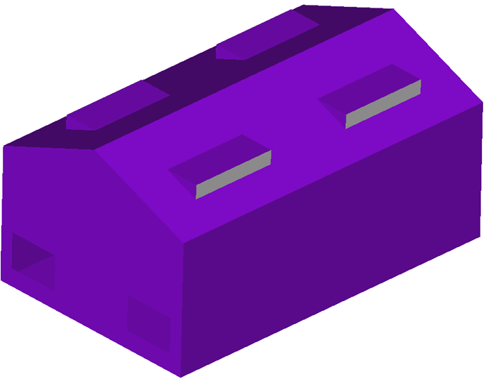
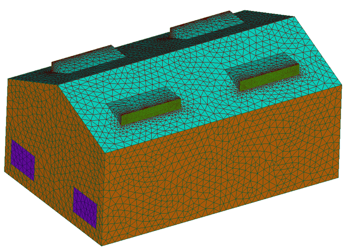
Examine the mesh in the modeling window. For the
purposes of this tutorial, the following steps lead to the display of inlet,
outlet and greenhouse walls.
Right-click Volumes > Display off.
Right-click Surfaces > Display on.
Right-click Surfaces > Display type > solid & wire.
Rotate, move or zoom the view to examine the mesh.
Figure 39. Mesh Details of the Geometry
Save the database to create a backup
of your settings.
Create the Thermal Shell and Assign Attributes
In the following steps you will generate the thermal shell, assign the number of
layers, material properties as well as radiation and solar radiation properties.
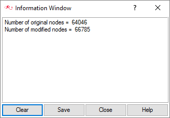
Under Surfaces, right-click on Roof and select Mesh Op. > Generate Thermal Shell.
An Information Window showing the number of
modified nodes is displayed. This will create a new volume set named
‘default_shell’ and new surface set named ‘default’. Figure 40.
The generated thermal shell will be exactly on the Top surface. Click
Display On and Display Off to
visualize the surfaces.
Rename the default surface to Shell_Top.
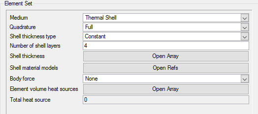
Double-click Element Set to open the detail panel.
Check that the Medium is set to Thermal Shell.
For Number of shell layers, enter 4.
Figure 41.
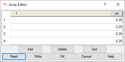
Next to Shell thickness, click Open Array to open the
Array Editor dialog to specify the thickness of each
shell.
Change the unit to cm and enter
0.25 for all the layers.
Figure 42.
Click OK to close the dialog.
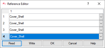
Next to Shell material models, click on Open Ref to open
the Reference Editor dialog to specify the material model
of each shell.
Note: You might get a warning stating that number of rows are less than the
table. Click Yes to add None as the default material
model for each shell.
Select the Cover_Shell as the material model for all the
layers by clicking on the drop down arrow.
Figure 43.
Click OK to close the dialog.
Under Surfaces, under Shell_Top, uncheck Simple Boundary Condition to disable
simple boundary condition for this surface.
Since this surface belongs to the ‘default_shell’ volume, Simple Boundary
Condition is disabled.
Click RAD in the Data Tree Manager.
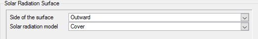
In the Data Tree, under Shell_Top, click the
Solar Radiation Surface check box to activate and open
the detail panel.
For Side of Surface, select Outward.
For Solar Radiation model, select Cover.
Figure 44.
Compute the Solution and Review the Results
Run AcuSolve
In the next steps you will run AcuSolve to compute the solution for this case.
Click on the toolbar to open the Launch
AcuSolve dialog.
Enter 4 for Number of processors, if your system has
four or more processors.
The use of multiple processors can reduce solution time.
Accept all other default settings.
Based on these settings, AcuConsole will generate
the AcuSolve input files, then launch the
solver.
Click Ok to start the solution process.
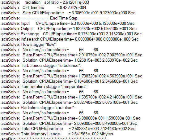
While computing the solution, an
AcuTail window opens. Solution progress is
reported in this window. A summary of the solution process indicates
that the run has been completed.
The information provided in the summary is based on
the number of processors used by AcuSolve.
If you use a different number of processors than indicated in this
tutorial, the summary for your run may be slightly different than the
summary shown.
Figure 45.
Close the AcuTail window and save the database to create a
backup of your settings.
Monitor the Solution with AcuProbe
While AcuSolve is running you can monitor the results
using AcuProbe.
Open AcuProbe by clicking on the toolbar.
In the Data Treeon the left, expand Residual
Ratio.
Right-click Final > Plot All.
The residual ratio measures how well the solution matches the governing
equations.
Note: You might need to click on the toolbar in order to properly display the
plot.
Figure 46.
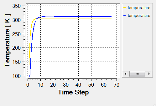
Post-Process with AcuProbe
The temperature on the roof of the greenhouse and the plant cover can be viewed at
the end of simulation using AcuProbe.
In the AcuProbe dialog, expand Radiation Output > Plant_Cover tri3 Greenhouse_Plants tet4 > Temperature.
Right-click on temperature and click
Plot.
Repeat the above steps for the Roof.
Figure 47.
View Results with AcuFieldView
Now that a solution has been calculated, you are ready to view the flow field using
AcuFieldView. AcuFieldView is a third-party post-processing tool that is tightly integrated to AcuSolve. AcuFieldView can be
started directly from AcuConsole, or it can be started
from the Start menu, or from a command line. In this tutorial you will start
AcuFieldView from AcuConsole after the solution is calculated by AcuSolve.
In the following steps you will start AcuFieldView to
display temperature on the plants and roof and heat flux on the roof of the
greenhouse.
Start AcuFieldView
Click on the AcuConsole toolbar to open the Launch
AcuFieldView dialog.
Click Ok to start AcuFieldView.
When you start AcuFieldView from AcuConsole, the results from the last time step of
the solution that were written to disk will be loaded for
post-processing.
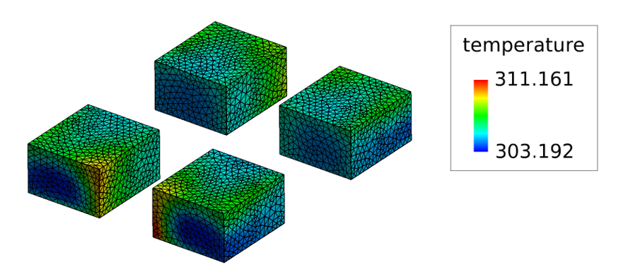
Create Boundary Surface Showing Temperature for the Plants
Click Viewer Options and uncheck the
Perspective check box to disable perspective view.
In the Viewer Options dialog, disable the axis
markers.
Orient the geometry so you can see inlet, outlet and greenhouse wall surfaces.
Click to open the Boundary Surface
dialog.
Check that Temperature is already selected as the Scalar Function.
Select the Plant_Cover tri3 Greenhouse_Plants tet4
surface from the Boundary Types list.
Click the Colormap tab and then select the check box for
Local to display the local range of values of
temperature for the selected surfaces.
Turn on the Legend on the Legends tab and change the
color to black from the color palette.
You can move the legend using Ctrl + left
click.
Change the annotation color to black.
Figure 48.
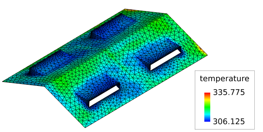
Create the Boundary Surface Showing the Temperature and Heat Flux for the Roof
In the Boundary Conditions dialog, select the
Shell_Top surface from the Boundary Types list.
Temperature should already be selected as the scalar function.
Figure 49.
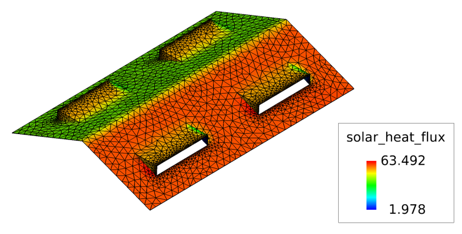
Click on Scalar Functions, and select Solar
heat flux.
Click Calculate to display the Solar Heat flux on the
roof.
Figure 50.
Summary
In this tutorial, you worked through a basic workflow to set up a steady state simulation
with solar radiation and thermal shell in a greenhouse. Once the case was set up, you
generated a mesh and generated a solution using AcuSolve. Then you
generated the thermal shell and assigned radiation properties to it. AcuProbe was used to post-process the temperature on the plant cover
and roof surfaces. Results were also post-processed in AcuFieldView to allow you visualize temperature contours on the plant
cover and roof, and heat flux values on the roof. New features introduced in this tutorial
include the solar radiation feature and thermal shell.

 on the
toolbar.
on the
toolbar.
 next to the item name.
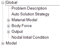
 on
the toolbar.
on
the toolbar.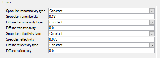

 and
and  next to the volume name.
Note: You may not see any change when toggling the display if Surfaces are being displayed, as surfaces and volumes may overlap.
next to the volume name.
Note: You may not see any change when toggling the display if Surfaces are being displayed, as surfaces and volumes may overlap.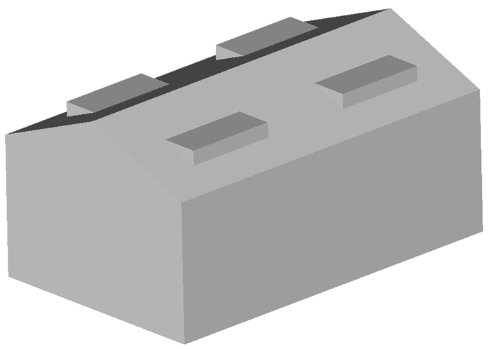

 on the toolbar to open the Launch AcuMeshSim
dialog.
on the toolbar to open the Launch AcuMeshSim
dialog.
 on the toolbar to open the Launch
AcuSolve dialog.
on the toolbar to open the Launch
AcuSolve dialog.
 on the toolbar.
 on the toolbar in order to properly display the
plot.
on the toolbar in order to properly display the
plot.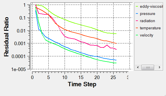
 on the AcuConsole toolbar to open the Launch
AcuFieldView dialog.
on the AcuConsole toolbar to open the Launch
AcuFieldView dialog.
 to open the Boundary Surface
dialog.
to open the Boundary Surface
dialog.